[模型推理] Inference From Scratch For GPT2 / 从头实现大模型的推理
文章含 AI 量:< 5%。AI 主要负责润色。
代码含 AI 量:< 5%。
代码面前,了无秘密。只有亲手重写一遍,才能看清藏在细节里的魔鬼。
代码: https://github.com/solofox/gpt2, branch: v1。
GPT2 是什么样的模型?
GPT2 是 OpenAI 在 2019 年开源的大语言模型,一个典型的 decoder-only 结构。用今天的眼光看,GPT2 的能力当然很初级——容易胡说八道,逻辑能力弱,连"法国的首都是哪个城市"都答不对。但它是 LLM 从"实验室玩具"走向"工业界基础设施"的关键催化剂:
- 伟大的试金石:它证明了 transformer 有能力处理长文本,不是只能玩机器翻译的小把戏。
- 商业化的破局者:巨头们彻底醒悟,随后引发了持续到现在的算力军备竞赛。
- 极佳的工程教材:结构足够简单,又足够完整,依然是学习 LLM 底层原理的最佳范本。
GPT2 官方一共发布了 4 个尺寸:gpt2-small / gpt2-medium / gpt2-large / gpt2-xl。它们都是 pretrained 模型,没有 instruction tuning。不像后来的模型系列——超大杯用 MoE 架构,中小杯用 dense 架构——GPT2 这几个尺寸除了超参数不同,网络结构完全一致。
参考
技术报告: https://cdn.openai.com/research-covers/language-unsupervised/language_understanding_paper.pdf
官方代码: https://github.com/openai/gpt-2.git。基于 tensorflow 1 写的,要在本机跑需要 python 3.6 及以下 版本。
参数一览:
| 变种 | d_model | 上下文窗口 | 层数 | 头数 | 参数量 |
|---|---|---|---|---|---|
| small | 768 | 1024 | 12 | 12 | 124M |
| medium | 1024 | 1024 | 24 | 16 | 355M |
| large | 1280 | 1024 | 36 | 20 | 774M |
| xl | 1600 | 1024 | 48 | 25 | 1.5B |
共同点:上下文窗口都是 1024,每个头的维度 d_k 都是 64。
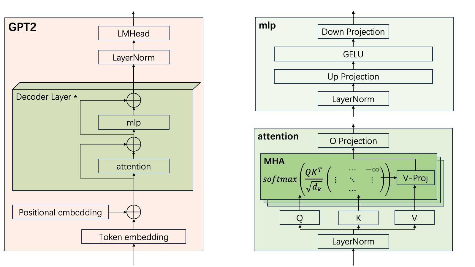
模型结构
技术报告里关于模型结构的描述,第一句就挺"坦诚"的——对不起,请回去看 Transformer 和 GPT1 的论文:
We use a Transformer (Vaswani et al., 2017) based architecture for our LMs. The model largely follows the details of the OpenAI GPT model (Radford et al., 2018) with a few modifications. Layer normalization (Ba et al., 2016) was moved to the input of each sub-block, similar to a pre-activation residual network (He et al., 2016) and an additional layer normalization was added after the final selfattention block. A modified initialization which accounts for the accumulation on the residual path with model depth is used. We scale the weights of residual layers at initialization by a factor of 1/√N where N is the number of residual layers. The vocabulary is expanded to 50,257. We also increase the context size from 512 to 1024 tokens and a larger batchsize of 512 is used.
结合 GPT1 技术报告里的描述:
Model specifications Our model largely follows the original transformer work [62]. We trained a 12-layer decoder-only transformer with masked self-attention heads (768 dimensional states and 12 attention heads). For the position-wise feed-forward networks, we used 3072 dimensional inner states. We used the Adam optimization scheme [27] with a max learning rate of 2.5e-4. The learning rate was increased linearly from zero over the first 2000 updates and annealed to 0 using a cosine schedule. We train for 100 epochs on minibatches of 64 randomly sampled, contiguous sequences of 512 tokens. Since layernorm [2] is used extensively throughout the model, a simple weight initialization of N(0, 0.02) was sufficient. We used a bytepair encoding (BPE) vocabulary with 40,000 merges [53] and residual, embedding, and attention dropouts with a rate of 0.1 for regularization. We also employed a modified version of L2 regularization proposed in [37], with w = 0.01 on all non bias or gain weights. For the activation function, we used the Gaussian Error Linear Unit (GELU) [18]. We used learned position embeddings instead of the sinusoidal version proposed in the original work. We use the ftfy library to clean the raw text in BooksCorpus, standardize some punctuation and whitespace, and use the spaCy tokenizer.
可以勾勒出 GPT1 的轮廓:
- 模型结构大部分跟《Attention Is All You Need》中的 transformer 一致。
- 位置向量是模型学习的,而不是原始论文中的正弦位置编码。
- 基础参数:L = 12, d_model = 768, h = 12, d_ff = 3072。
- 正则化用 LayerNorm。
- 激活函数用 GELU。
- tokenizer 用 BPE 编码。
GPT2 相比 GPT1,只改了三处:
- LayerNorm 从每个子层的后面移到了前面(原因论文里没解释,但跟 pre-activation residual network 的设计思路一致)。
- 在最后一个 attention block 之后,额外加了一个 LayerNorm。
- 词汇表大小 V = 50257;上下文长度翻倍到 1024。
整体结构画出来是这样的:
代码实现
只要熟悉 PyTorch 里模型的写法,GPT2 的代码并不比 MNIST 复杂太多。只是有些操作在图像处理中不常见,写法上需要花点时间适应。
下面聊聊我在写的过程中花了一些时间的地方。
safetensors 文件格式
safetensors 的文件格式挺直观的:文件头是一个 JSON,描述了里面存了哪些 tensor 以及各自的形状和数据类型。大部分加载逻辑都很直白,唯一的问题是:怎么把存储的浮点数数组转成 torch.tensor?答案是用 torch.frombuffer:
# utils.py:_load_tensor
tensor = torch.frombuffer(bytearray(buffer), dtype=dtype).reshape(shape)
反过来,把 tensor 存成 bytearray 用 tensor.numpy().tobytes():
if not tensor.is_contiguous():
    tensor = tensor.contiguous()
bytes = tensor.numpy().tobytes()
Embedding 查找
输入: input_ids,形状 [B, N](B=batch_size, N=seq_len)
词嵌入: wte,形状 [V, d_model](V=vocab_size);位置嵌入: wpe,形状 [L, d_model](L=max_context_window)
目标: 把 input_ids 里的每一个 token id 映射成对应的 embedding 向量,最终输出形状 [B, N, d_model]。
用 tensor 做索引这个语法,一开始可能不太习惯,但其实非常简洁:
# 词嵌入:直接用 token id 查表
wte[input_ids]  # → [B, N, d_model]

# 位置嵌入:用位置序号查表,而不是 token id
positions = torch.arange(0, input_ids.shape[-1], dtype=torch.long, device=input_ids.device)
wpe[positions]  # → [N, d_model]
这是 PyTorch 的高级索引语法,以后可以专门写篇小文章展开讲。
Attention
一开始我写 Attention 是老老实实按头循环的:
def attention(self, x: torch.Tensor) -> torch.Tensor:
    seq_len = x.shape[-2]

    x = F.layer_norm(x, normalized_shape=(self.d_model,), weight=self.ln_1_weight, bias=self.ln_1_bias, eps=self.layernorm_eps)

    scale = torch.rsqrt(torch.tensor([self.d_model / self.h], dtype=x.dtype, device=x.device))

    qkv_merged = torch.matmul(x, self.attn_weight) + self.attn_bias
    qkv_split = torch.split(qkv_merged, self.d_model // self.h, dim=-1)
    assert len(qkv_split) == 3 * self.h

    q_split = qkv_split[ : self.h]
    k_split = qkv_split[self.h : 2 * self.h]
    v_split = qkv_split[2 * self.h : ]

    heads = []
    for i in range(self.h):
        qk_similarities = torch.matmul(q_split[i], k_split[i].transpose(-2, -1)) * scale
        qk_similarities += self.causal_bias[:seq_len, :seq_len]
        qk_similarities = F.softmax(qk_similarities, dim=-1)
        head_i = torch.matmul(qk_similarities, v_split[i])
        heads.append(head_i)
    x = torch.concat(heads, dim=-1)
    x = torch.matmul(x, self.attn_proj_weight) + self.attn_proj_bias
    return x
GPT2 里,QKV 的映射矩阵是合并成一个大矩阵的,形状为 [d_model, 3 × d_model]:
- [d_model, 0 : d_model] 是 Q 的映射矩阵
- [d_model, d_model : 2 × d_model] 是 K 的映射矩阵
- [d_model, 2 × d_model : 3 × d_model] 是 V 的映射矩阵
GPT2 中 d_k = d_model / h,所以上述操作的过程是:
x = x @ W_QKV + B_QKV,得到 [B, N, 3 × d_model]- 把 x 的最后一维按 d_k 切分,得到一个 list,共 3×h 个元素,每个形状 [B, N, d_k]
- 排列顺序:
[q_0, q_1, ..., q_{h-1}, k_0, k_1, ..., k_{h-1}, v_0, v_1, ..., v_{h-1}] - 循环取出 q_i, k_i, v_i,计算 attention:
softmax(causal_mask(q_i @ k_i^T / sqrt(d_k))) @ v_i - 拼接所有头的结果
这里的问题是:第 3 步和第 4 步不匹配——第 4 步需要的 q_i, k_i, v_i 在 list 里并不连续。如果能重新排列成:
[q_0, k_0, v_0, q_1, k_1, v_1, ..., q_{h-1}, k_{h-1}, v_{h-1}]
那就顺手多了。
后来参考 GPT-2 官方代码,用纯矩阵操作替代了循环,代码干净了很多:
def attention(self, x: torch.Tensor) -> torch.Tensor:
    seq_len = x.shape[-2]

    x = layer_norm(x, weight=self.ln_1_weight, bias=self.ln_1_bias, eps=self.layernorm_eps)
    qkv_merged = torch.matmul(x, self.attn_weight) + self.attn_bias

    scale = torch.rsqrt(torch.tensor([self.d_model / self.h], dtype=x.dtype, device=x.device))

    # split q, k, v
    q, k, v = qkv_merged.split(self.d_model, dim=-1)
    q = q.reshape((-1, seq_len, self.h, self.d_model // self.h))
    q = q.transpose(-2, -3)
    k = k.reshape((-1, seq_len, self.h, self.d_model // self.h))
    k = k.transpose(-2, -3)
    v = v.reshape((-1, seq_len, self.h, self.d_model // self.h))
    v = v.transpose(-2, -3)

    scores = torch.matmul(q, k.transpose(-2, -1)) * scale
    # causal mask
    scores += self.causal_bias[:seq_len, :seq_len]
    scores = F.softmax(scores, dim=-1)
    scores = torch.matmul(scores, v)
    # merge back
    x = scores.transpose(-2, -3)
    x = x.reshape((-1, seq_len, self.d_model))

    x = torch.matmul(x, self.attn_proj_weight) + self.attn_proj_bias
    return x
关键的四步变换:
- Q/K/V 各自是 [B, N, d_model]
- 按注意力头拆分词向量:
reshape→ [B, N, h, d_k]。此时不同头在第三维上交叉排列 - 交换 N 和 h 的维度:
transpose→ [B, h, N, d_k]。这样同一个头所有词的词向量就构成了一个连续矩阵,维度 N 是序列长度,d_k 是头的维度 - 按单头方式批量计算 attention,最后逆向合并回来
心得
整体的细节其实不少,我最后是对着官方 tensorflow 1 的代码一行一行分析,才把代码跑顺的。以下是几个踩坑后总结的经验。
矩阵结构要时刻刻在脑子里
每一步操作,都注释好各操作数的矩阵结构:有几维,每一维大小是多少。调试时遇到 shape 不匹配的异常,第一时间把 shape 打印出来看看。
对于 reshape、transpose、split 等操作,要经常翻文档确认——它操作的是哪一维?维度是合并还是分裂?对 dim 和 keepdim 这两个参数保持敏感。
行向量 vs 列向量
看公式或论文时,要搞清楚数学上的向量约定和代码实现之间的差异。
数学上大部分用列向量,写法是 W @ x。但在代码实现中,几乎全部用行向量,写法是 x @ W。
即使都是行向量,W 用的是原始矩阵还是转置矩阵,也要分清楚。在 GPT2 中,权重矩阵的维度是 [in_features, out_features],跟数学上的维度一致。但在 PyTorch 的 nn.Linear 中,默认存的是 [out_features, in_features]。这一点如果不注意,矩阵乘法就会静默地算出错误结果。
调试方法
我的调试策略很直接——跟官方实现逐层对比:
- 在我的每个操作之后,把结果写入文件系统,存成 safetensors 格式
- 写一个对比工具,分别读入我的结果和官方结果
- 用二分法缩小范围,定位到具体哪个操作有偏差
- 搜索这个操作的具体原理
- 如果还搞不定,直接看官方实现
这个方法虽然笨,但是极其有效。
Stay curious
从今天的视角看,这个模型挺傻的。
它连"法国的首都是哪个城市"都答不对:
harry$ python ./main.py ./models.cache/gpt2-small/ "Which city is the capital of France"
?

Some people think they have a lot in common. They both inherited the country from the French Revolution, so they won't be as happy about their own future as their French counterparts.

What about the rest of France? How does France's economy plan to cope with a 20% growth rate next year?

France has been experiencing a steady decline in its exports. It's not about to stop, as the IMF and European Central Bank have recently said. In fact, this is a political decision which many believe will be made by France's leaders. The political leaders of the European Union are going to be much stronger.
它听不懂人类的指令。它喜欢写故事——不管你输入什么,它都把它当成故事的开头,然后不停地往下续写。这就是 pretrained 模型和 instruction 模型的本质区别:
harry$ python ./main.py ./models.cache/gpt2-small/ "Say you love me once and stop immediately"
, cuz I'm not gonna stop you."

But then she turns to him, and he says, "Well, I just gave you a couple of dollars. I've got a few more."

"You're not taking that," he says, "I'm just giving you a couple dollars, when you've got all these resources and you've just got to be willing to let me say something, you know?"

So she says, "I know you love me, but I just want to know, what are you going to do?"

"I'm not doing anything," he says, and she says, "I'm just starting to make my financial situation better."

"Yeah, that's fine," she says.

"How about you give me some $10,000?"

"Well, I'll give you a^C
Aborted!
贪婪采样(top-k=1)很容易就陷入死循环:
harry$ python ./main.py ./models.cache/gpt2-small/ "Do you love me?" -k 1
 I love you. I love you. I love you. I love you. I love you. I love you. I love you. I love you. I love you. I love you. I love you. I love you. I love you. I love you. I love you. I love you. I love you. I love you. I love you. I love you. I love you. I love you. I love you. I love you. I love you. I love you. I love you. I love you. I love you. I love you. I love you. I love you. I love you. I love you. I love you. I love you. I love you. I love you. I love you. I love you. I love you. I love you. I love you. I love you. I love you^C
Aborted!
但正因为这个模型足够简单、足够"傻",它才是一面完美的镜子——让你看清一个语言模型到底在做什么,而不会被各种花哨的 RLHF、MOE、KV cache 优化分散注意力。
如果你也想亲手拆开一个 LLM 看看里面长什么样,GPT2 是最好的起点。